The first two topics covered in Quantitative Methods of Ed Tech are simple and multiple regression. These two topics are ones I not only have covered before, but also spent time reviewing recently so they were very fresh in my mind.

Starting with these topics was an excellent confidence booster and, although I found Field’s description of these concepts in Chapter 8 and 9 slightly difficult, the recorded lecture and labs answered any questions I had. In particular, the lab’s brief overviews of the lectures’ key topics before going into the lab exercises were particularly helpful and worth listening to more than once.

As these topics were easier for me, my notes on simple and multiple regression will focus on the most important takeaways and any additional resources I used.

Simple Regression

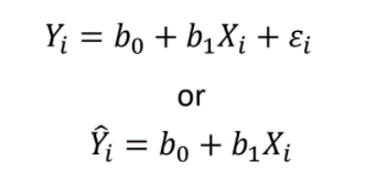
To begin, regression is a statistical procedure used to provide a standardized method for determining the best-fitting straight line to any set of data. This linear relationship between two variables can be expressed by the equation:

Where b₀ is the Y-intercept and b₁ is the slope (regression) coefficient. The slope determines how much Y will change for every change in X.

The linear equation is used to determine a Y value on the line: the predicted Y or Y-hat.

One thing to note is that the regression line is only a model based on data. In other words, it may not reflect reality. Basically, analysis of regression is used to test the significance of a regression equation. If analysis of regression shows the model does not fit reality, then the model is not helpful in understanding why the Y values are different/vary.

The sum square model examines the total variabilities:

Once the sum of squares are found, the mean squares can be attained (i.e., the variance accounted for by the regression model and the variance explained by the residual model) and an F-ratio can be used to compare the two mean squares. With the F-ratio, whether the statistic is significant can be determined.

Multiple Regression

Multiple regression is similar to simple regression except it uses several predictor variables to predict Y. The reason for selecting multiple regression is that using two or more predictor variables can help to obtain more accurate predictions of Y.

In multiple regression equations, the regression coefficients each represent the unique contributions of an X variable after all other X variables have been controlled.

There are three methods of regression: forced entry, hierarchical, and stepwise. These methods describe when predictors are entered into the regression model.

For forced entry, all predictors are entered at the same time. To use this method, it is important to consider each variable and why it is being included in the model.

In hierarchical regression, the researcher first enters known variables that have shown a correlation in previous research. Then new variables are entered to test their unique contribution to the model. This type of regression is often used for theory testing.

Finally, stepwise regression is used for exploratory research. In this case, predictor variables are entered based on which can explain the most variance first and, if a variable is significant, additional variables will continue to be selected and added to the model. Basically, how much more variance can be explained is being looked at and if R² significantly increases then keep going.

Bias in Regression Model

When working with regression models, one must be aware of bias: outliers, sample size and model assumptions not being met.

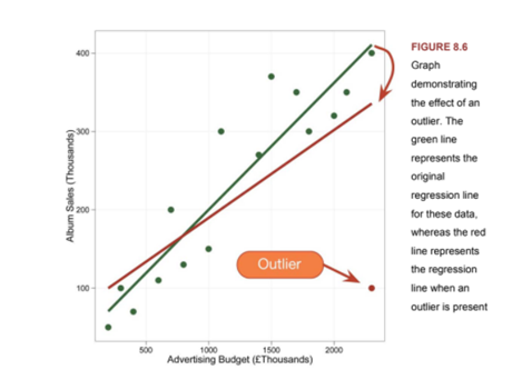
Outliers, for example, can significantly affect a regression line.

In the case of sample sizes, the number of predictors and the size of the expected effect should be considered when determining the sample size required to test the overall regression model.

In terms of assumptions, predictors must not have zero variance, the relationship between the X and Y variables must be linear, error terms should be uncorrelated and normally distributed, there should be no multicollinearity, homoscedasticity should be met, and the outcome scores should all come from independent individuals (i.e., individuals in the sample should not be affecting each other).

Reporting

When reporting a regression model, whether the overall regression equation was statistically significant should be included, as well as how well scores on the Y variable can be predicted. In addition, the p-value should be stated.

Key Terms

• Multicollinearity: predictors should add uniqueness to a regression model and, as such, predictors should not be highly correlated
• Homoscedasticity: for each value of the predictors the variance of the error term should be constant

Additional Resources

• Simple Regression: https://www.statisticshowto.com/probability-and-statistics/regression-analysis/find-a-linear-regression-equation/
• Multiple Regression: https://www.statisticshowto.com/probability-and-statistics/regression-analysis/
• Multiple Regression: https://youtu.be/dQNpSa-bq4M

References

Anderson, D. R., Sweeney, D. J., Williams, T. A., Camm, J D., & Cochran, J. J. (2018). Statistics for Business & Economics (13th ed., revised). Cengage Learning.

Field, A. (2017). Discovering statistics using IBM SPSS statistics (5th ed.). SAGE Publications.

Howell, D. C. (2017). Fundamental Statistics for the Behavioral Sciences (9th ed.). Cengage Learning.